This page teaches users how to genotype a molecular marker, how to organize genotypic data for analysis with Joinmap and MapMaker software, and how to test whether genotypic data meets an expected segregation pattern using the chi-square test. Sample data is provided.
Learning Objectives
At the end of this lesson you should:
- Be familiar with the conventional layout of an agarose gel photo;
- Be able to score genotypic data; and
- Be able to organize genotypic data in a Microsoft Excel spreadsheet.
Introduction
The purpose of this article is to provide an example of how to genotype individual tomato plants with a molecular DNA marker. There are several different molecular marker systems available to assist plant breeding programs. For the purposes of this lesson, the marker chosen as an example is a cleaved amplified polymorphism (CAP) marker, a type of marker that is often visualized by gel electrophoresis. Briefly, a CAP marker exploits differences in DNA sequences between two polymerase chain reaction (PCR) products based on the presence or absence of restriction enzyme cutting sites found within that segment of DNA. To genotype a CAP marker, the segment of DNA is amplified using PCR then cut with a restriction enzyme (referred to as digestion, or restriction enzyme digestion), which only cuts at a specific DNA sequence. After digestion, the DNA is separated on agarose gel. CAP markers are designed so that the restriction enzyme will cut the DNA of one genotype, but not another.
Although different breeding program schemes can be used, in this particular case, the individual plants are from an F2 population that is segregating for the marker. In all breeding programs, the specific marker being used must be segregating among the plant population being used in order to be useful.
CAP markers are generally visualized using gel electrophoresis. When scoring any molecular DNA marker using gel electrophoresis, keep the following considerations in mind:
- Include a molecular weight ladder. This is like a DNA size ruler that contains DNA fragments of known molecular weight in base pair length (Fig.1). Since many markers are scored based on their molecular weight in DNA base pairs (bp), this ladder is essential to determine the molecular weight of each band in a gel
- Include controls. In addition to the individuals being genotyped, individuals of known genotype (often the parents of the population) should be included to make sure to identify the correct bands in the gel to score in the population.
- Know the characteristics of the molecular DNA marker in the germplasm you are using. Important attributes include the expected banding pattern (one band or multiple bands), the molecular weight of each segregating band, if the marker is dominantly or codominantly inherited, and so forth.
All these considerations will make it easier to score a marker from a gel photo. Next we will follow a specific CAP marker example in a tomato breeding program.
Genotyping Example
The gel photo below (Fig.1) is a CAP marker, CosOH57, genotyped in 30 individuals that were part of a larger F2 population developed from the parents OH88119 and 06.8068. The population was developed as part of a breeding project to incorporate bacterial spot resistance into elite germplasm. In order to score the gel, the bands are evaluated based on the considerations listed above:
- Molecular weight ladder. The ladder is in lane 1 and is a 100 base pair ladder.
- Controls. The parents of the cross are included in the gel photo in lanes 2 and 3; they provide a reference for the F2 plants. Notice the difference in banding patterns between the two parents, with OH88119 showing a band at 216 bp and 06.8068 showing two bands, one at 145 bp and another at 71 bp. These are the bands we will follow in the 30 F2 progeny (Fig. 1).
- Marker characteristics. As we described above, CAP markers must be amplified using PCR and then digested with a restriction enzyme. In this case, the PCR products for the parents OH88119 and 06.8068 have the same molecular weight (216 bp). However, after restriction enzyme digestion with restriction enzyme, Tth111I, the PCR product from OH881119 is not cut (and remains 216 bp long), whereas the PCR product from 06.8068 is cut into two pieces of 145 and 71 bp. Like most CAP markers, CosOH57 is codominant. In heterozygous individuals, the OH88119 allele will not be digested, producing the 216 bp band, but the 06.8068 allele will produce the two smaller bands, so all three bands are present after digestion.
- The individuals in lanes 4 through 33 are part of an F2 population derived from crossing OH88119 and 06.8068. The 30 F2 individuals genotyped with CosOH57 should segregate in a 1:2:1 ratio (homozygous for parent A allele : heterozygous: homozygous for parent B allele). Think of it like a simple Aa x Aa selfing of F1s to give 1AA: 2Aa :1aa in the F2 generation.
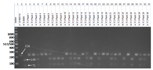
Figure 1. Example gel photo of CAP marker CosOH57. The gel includes a DNA ladder, the parental genotypes (OH88119 and 6.8068), and 30 F2 individuals. Photo credit: Matthew Robbins, The Ohio State University.
Scoring the Gel
Knowing the information outlined above, the gel can be scored. Most computer programs that use marker data in subsequent analyses have a specified data format. For segregating populations, many programs code the data in relation to the parents. For example, Joinmap and MapMaker, two programs that are commonly used for mapping, code genotypes from an F2 population as follows:
Table 1: Genotype codes for an F2 population.
| Code |
Genotype |
| A |
homozygous for parent 1 allele |
| B |
homozygous for parent 2 allele |
| H |
heterozygous |
| C |
not genotype A (dominant B allele, so could be a genotype like parent 2 or heterozygous) |
| D |
not genotype B (dominant A allele, so could be a genotype like parent 1 or heterozygous) |
| “.” |
genotype unknown (missing data) |
Keep in mind the following when scoring the genotypes:
- The determination of which parent is “parent 1” or “parent 2” is arbitrary. BUT the parental designation MUST be consistent for all markers scored on the same population. In this example, OH88119 is parent 1 (coded as A) for CosOH57, so OH88119 MUST also be parent 1 for all other markers on this population.
- The A, B, and H codes are applied to codominant markers, while A and C (parent 2 allele is dominant) or B and D (parent 1 allele is dominant) codes are for dominant markers.
- It is also important to code for unknown or missing data—a period, in this example.
Using the genotypic codes, each individual tomato plant is scored (Fig. 1). In the example we are following, CosOH57 is a codominant marker, so the 30 F2 individuals are coded as “A” when only the 216 bp band is present, “B” when a plant has both the 145 and 71 bp bands present, or “H” when all three bands are showing for an individual tomato plant.
Genotypic scores can also be coded by the molecular weight of the fragment. This is useful when genotyping a set of individuals without common parents, and especially if multiple alleles of the marker are present. In this simpler CosOH57 example, using the molecular weight scoring method, parent 1 would be scored as “216” and parent 2 could be scored as either “145” or “71.”
Organizing Genotypic Data
Once the molecular marker is scored, it is useful to organize the data in a spreadsheet or table format. This allows data from other markers genotyped in the same population to be combined in preparation for mapping or other analyses. The individual genotypes for CosOH57 have to be reorganized into a table with markers as rows and individual plant genotypes as columns (Table 2). It is important that “F2 Plant #1” is always the same plant, no matter the particular marker being genotyped. This is a common format for mapping software. The rows for Marker2 and Marker3 indicate that genotypic data can be added for additional markers. Although parental genotypes are not included in mapping analysis, it is useful to keep them with the data for reference.
Table 2. Table with genotypic data organized with markers as rows and individual genotypes as columns.
| Marker |
OH88119 |
6.8068 |
F2 Plant 1 |
F2 Plant 2 |
F2 Plant 3 |
… |
| CosOH57 |
A |
B |
A |
A |
H |
|
| Marker2 |
|
|
|
|
|
|
| Marker3 |
|
|
|
|
|
|
| … |
|
|
|
|
|
|
Data Verification by Chi-square Test
Data summaries are also useful to check whether the data collected seems reasonable based on what you expect for a particular population, or if something else may be going on, such as the marker being linked to a trait we are selecting for or forces such as natural selection are distorting the expected segregation pattern. In our example, we may want to verify that the CosOH57 marker genotypes segregate as expected—1:2:1—using a chi-square goodness-of-fit test (note: For a refresher on how to use chi-square, you may want to take a look at the chi-square lesson). The data for the gel photo above, not including the parents, is summarized in Table 3. The observed column is determined simply by counting the number of individual plants with each genotype. The expected number of each genotype is calculated by multiplying the expected frequency of the genotype by the total number of plants being genotyped:
Expected = Expected Frequency x Total
The expected frequency is determined based on the segregation ratio of 1:2:1 for our F2 population, which is 0.25: 0.5 :0.25. Thus, the expected frequency of the “A” genotype for CosOH57 is:
Expected “A” Genotype = Expected Frequency of “A” Genotype x Total Number of F2 Plants Being Genotyped
or
Expected “A” Genotype = 0.25 x 30 = 7.5
The expected frequencies and number of each genotype are also presented in Table 3.
Table 3: Summary of the CosOH57 F2 gel data.
| Genotype |
Observed |
Expected frequency |
Expected |
| A |
13 |
0.25 |
7.5 |
| B |
7 |
0.25 |
7.5 |
| H |
10 |
0.5 |
15 |
| Total |
30 |
1 |
30 |
When the observed and expected numbers are used in a chi-squared goodness-of-fit test, the calculated p value is 0.057. Since this p value is a little greater than 0.05, a common level to declare significance, there is some evidence that CosOH57 may segregate as expected. Closer inspection of the data indicates that the actual observed frequency of genotype “A” may be higher than expected, while the H genotype may be lower than expected. Additional caution should be exercised because the relatively small number of F2 individuals make it difficult to interpret this chi-square test. Ideally, statisticians recommend genotyping an F2 population using at least 50 individuals.
Conclusion
In this tutorial we learned how to genotype a CAP marker that was scored in an F2 population. The principles we used apply to any other molecular marker that we may genotype, particularly molecular markers genotyped on a gel. These general principles also apply to other plant breeding schemes. We also learned how to organize data so that we can use it for genetic mapping. Finally, we learned how to perform a chi-square analysis as an additional test to help us determine the reliability of a specific marker in our breeding population.
External Links
Additional Resources
For additional practice scoring an agarose gel:
Funding Statement
Development of this page was supported in part by the National Institute of Food and Agriculture (NIFA) Solanaceae Coordinated Agricultural Project, agreement 2009-85606-05673, administered by Michigan State University. Any opinions, findings, conclusions, or recommendations expressed in this publication are those of the author(s) and do not necessarily reflect the view of the United States Department of Agriculture.
PBGworks 659