
Author:
Shawn Yarnes Ph.D., The Ohio State Univeristy
Objectives
- Estimate the sample size required to differentiate two means
- Estimate the minimum detectable difference between two means dictated by a given sample size
- Understand the relationship between sample size, error, and minimum detectable difference
N = [(4σ2)(Z(1-(α/2)) + Z(1-ß))2] ÷ E2
N = total sample size (number of experimental units within both treatments)
σ = assumed standard deviation of each treatment response (both treatments assumed equal)
Z(1-(α/2))= related to the chosen significance criterion α; can be found in normal distribution tables, or calculated in Microsoft Excel using the formula = NORM.S.INV(1- (α/2)
Z(1-ß)= related to the chosen power, or sensitivity of the experiment; can be found in normal distribution tables, or calculated in Microsoft Excel using the formula = NORM.S.INV(1-β)
E = minimum detectable difference between treatment means
To solve the equation for total sample size you first must assign a priori values. The variables, Z(1-(α/2) and Z(1-ß) are set based on acceptable confidence and power levels, generally determined by scientific discipline. The variable, σ, is the assumed standard deviation of treatment based on prior knowledge, measured either from a pilot or preliminary study or from previous work, and E is the magnitude of the difference the investor hopes to be able to statitisically differentiate in the experiment. Once these four a priori values are set, the total sample size, N, can be calculated.
Steps to Solve Equation
- To determine Z(1-(α/2) you must choose an acceptable confidence level. The minimum confidence level accepted in science is 95%. Setting the confidence level to 95% means that the investigator is willing to accept a 5% chance that a statistical test will generate a false positive result, or Type-1 error. The significance criterion for a 95% confidence level is denoted as, α = 0.05. The value corresponding to α = 0.05 is 1.96.
- To determine Z(1-ß) you must choose the sensitivity, or power, of your experiment. A power of 90% means that the investigator is willing to accept a 10% chance that a statistical test will generate a false negative result, or a Type-2 error (ß). The value corresponding to ß = 0.10 is 1.28.
- Set a value for the ideal level of minimum detection. Assume that the investigator would like to detect a difference of 0.5g in dry weights between two treatments (E = 0.5).
- The final step is to develop the estimate of error, standard deviation (σ), that might reasonably be expected in the experiment, either from a preliminary experiment or from previous similar studies. Assume that you have the results of a small-scale (Table 1) pilot study. Individual plants representing the eventual control treatment were grown under similar conditions as the anticipated large-scale experiment, and their dry weights recorded in the table below. From these values the standard deviation can be calculated. Standard deviation is the degree to which individuals within the sample differ from the sample mean. In this case σ = 5.88.
| Dry Weight (g) |
|---|
| 48.6 |
| 43.0 |
| 50.1 |
| 36.3 |
| 39.4 |
Table 1: Preliminary Results (n = 5)
N = [(4)(5.88)2) (1.96 + 1.28)2 ] ÷ (0.5)2 = 5,807
In this example the investigator would need to have treatment sizes of n = 2,904 plants (n = N ÷ 2 ) to detect a 0.5g difference between treatments.
Solving for Minimum Detectable Differences
E = √[(4σ2 (Z(1-(α/2)) + Z(1-β)) 2) ÷ N]
Consider that the investigator has learned that greenhouse space is limited to only 300 plants. The equation can be rearranged to determine the minimum detectable difference between treatment means for N=300.
E = √[(4) (5.9)2 (1.96 + 1.28) ÷ 300] = 2.2
Given the space constraints and the estimated standard deviation, the minimum difference that can be detected with 300 plants is 2.2g dry weight.
Relationship Between Sample Size, Minimum Detectable Difference, and Error
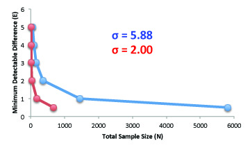
As sample size increases the minimum difference that can be detected increases, but at a diminishing rate. The most effective way to reduce sample size is to reduce error. The blue line represents the standard deviation of plant dry weights observed in the previously mentioned pilot study (σ = 5.9). To detect a 1g difference in dry weights between the two treatments requires a total sample size of 1,454. The red line represents a smaller error measurement of σ = 2.00, that could perhaps be obtained by growing clonal plants instead of siblings. With less variation, the total sample size needed to detect a 1g difference in dry weight is only 168 plants.
Additional Resources
Many statisitics text books provide detailed explainations of sample size estimations:
Kuel, R.O. (2000) Design of Experiments: Statistical Principles of Research Design and Analysis, 2nd Duxbury Press, Pacific Grove.
Related eXtension Plant Breeding and Genomics Resources:
Equation to Estimate Sample Size Required for QTL Detection
Gene Pyramiding Using Molecular Markers
Funding Statement
Development of this page was supported in part by the National Institute of Food and Agriculture (NIFA) Solanaceae Coordinated Agricultural Project, agreement 2009-85606-05673, administered by Michigan State University. Any opinions, findings, conclusions, or recommendations expressed in this publication are those of the author(s) and do not necessarily reflect the view of the United States Department of Agriculture.
PBGworks 1430