Category: Plant Breeding Genomics

This session will focus on highly parallel genotyping tools. We are moving away from scoring sequence polymorphism as a “band on a gel”. We will present the design of the SolCAP/Illumina consortium tool, discuss the resulting data format, and discuss quality control.

You can view the webinar below or at the SolCAP website.

View the webinar transcript.

If you experience problems viewing this video connect to our YouTube channel or see the YouTube troubleshooting guide.

 Presenter: Allen Van Deynze, University of California, Davis

View other SolCAP webinars

External Links

• Van Deynze, A. 2010. Working with Infinium genotype data. [Online seminar]. Solanaceae Coordinated Agricultural Project. Available at: solcap.msu.edu/infinium_genotype_webinar.shtml (verified 11 May 2012).

Funding Statement

Development of this page was supported in part by the National Institute of Food and Agriculture (NIFA) Solanaceae Coordinated Agricultural Project, agreement 2009-85606-05673, administered by Michigan State University. Any opinions, findings, conclusions, or recommendations expressed in this publication are those of the author(s) and do not necessarily reflect the view of the United States Department of Agriculture.

Mention of specific companies is not intended for promotional purposes.

PBGworks 884

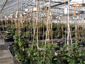
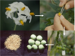
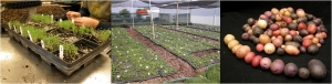
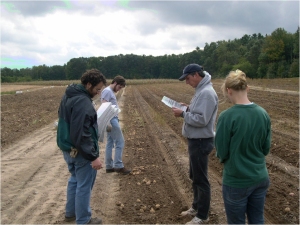
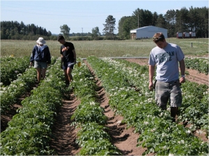
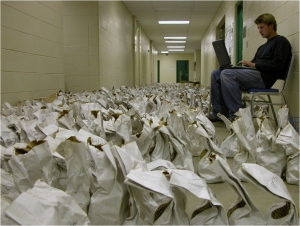
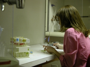
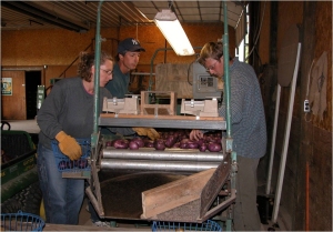
Photo credit: Patrick Hayes, BarleyWorld.org, Crop and Soil Science Department, Oregon State University

In the United States, barley is grown in 25 states, but the bulk of the production is in seven states. Each of these states hosts at least one checkoff organization, which collects money from producers to promote and support barley production, marketing, and research. As with most crops, certain information is critical for growers to optimize their chances to maximize production. Organizations, universities, and affiliated research and extension centers in each state provide such information on optimal variety selection, as well as state-specific information on marketing; economics; and prevalent diseases, insects, and weeds.

• Idaho
• Minnesota
• Montana
• North Dakota
• Washington
• Maryland
• Oregon
• Wisconsin
• United States

Idaho

Idaho Barley Commission is a self-governed state checkoff organization that works for Idaho barley producers to improve production and profitability of barley in the state. This site provides information on management practices, market reports, newsbriefs, nutrition, and publications.

Idaho Grain Producers Association represents Idaho grain producers at county, state, and federal levels to ensure the viability and profitability of their farming operations. This site provides information on markets, research, and state agricultural agencies, and it links to the Idaho Grain Magazine.

University of Idaho Extension. Provides information on crops, fertilizers and soils, direct seeding and conservation tillage, and pests and pesticides. This site also has information on insect pollinators and irrigation.

USDA/ARS Aberdeen National Small Grains Collection. Maintains collections representing global diversity of small grains, including barley. The site houses the Barley Genetic Stock Collection, which contains over 2,000 germplasm lines of diverse geographic origin.

Minnesota

The Minnesota Barley Research and Promotion Council is a state checkoff organization that works with Small Grains.org to support barley research and interests. The Small Grains site provides information on markets, policy, and production issues.

University of Minnesota Agricultural Experiment Station is responsible for up-to-date research information, showcasing yearly evaluations of yield, agronomic, and disease characteristics of multiple barley varieties in Minnesota.

Montana

Montana Wheat and Barley Committee is a Montana Department of Agriculture organization, funded and directed by producers through a checkoff program. Their goal is to protect the interests and viability of wheat and barley production in Montana. The site provides information on rail rates, weather, and news.

Montana Grain Growers Association is an association of grain producers that works to represent Montana grain growers through legislation efforts that affect farming. This site contains information on policy, research, news, and local events.

Montana State University Agricultural Research Centers are located throughout the state. This site provides localized information on research related to varieties, pest and disease control, and other barley production issues. 

North Dakota

North Dakota Barley Council is a producer-run organization, supported by checkoff funds, that provides information on barley utilization, research, marketing, and legislation. North Dakota is the top-ranked barley production state in the U.S.

North Dakota Grain Growers Association provides marketing and weather information, as well as the Gleaning newsletter, which contains information on grain yields, market prices, and other regional information of interest to growers.

NDSU Agricultural Experiment Station provides information on variety trial results, insect pest reports and management recommendations, and information on weeds and weed resistance.

North Dakota Irrigation Association has a publication that provides recommendations for irrigated malt barley production. Posted with permission by North Dakota Irrigation Association.

Institute of Barley and Malt Sciences. This institute provides information on the 2008, 2009, and 2010 American Malting Barley Association (AMBA) list of approved malting barley varieties. A detailed malting production calendar is also available.

Washington

Washington Grain Alliance provides funded research project summaries, as well as marketing and general crop information.

Washington State University Cereal Variety Testing Program provides weather data, variety brochures, and monthly rust updates.

Maryland

Maryland Grain Producers provides information on their checkoff grant program, general information on biofuels, and a speakers bureau established to raise awareness of agriculture.

University of Maryland’s Research and Extension Centers provide information on the use hulless barley for ethanol production and screening barley cultivars for ethanol production.

Oregon

Barley World, operated out of Oregon State University, offers an image gallery, information on barley food and straw and winter malting/food/forage barley breeding.

Oregon Wheat Growers League provides up-to-date local weather conditions.

Oregon State University, Crop and Soil Science Department barley page. This site contains information on varieties, diseases, nutrient management, and weeds.

Wisconsin

USDA-ARS-Cereal Crops Research Unit, located in Madison, WI. This site contains information about research programs and projects, barley quality analysis, and news.

United States

National Barley Growers Association is a national barley advocacy organization that works to ensure that US barley producers’ concerns are heard both nationally and internationally. This organization works closely with federal policymakers, congressional offices, and regulatory agencies to ensure barley producers’ concerns are addressed.

National Barley Improvement Committee is a national coalition representing barley producers, researchers, and end-users that works to address and discuss important national and regional barley research issues, and to ensure adequate funding for these areas. This site provides data on the economic significance of barley.

U.S. Grains Council is a private, nonprofit organization that works to build export markets for barley, corn, and sorghum. This site provides a database of grain suppliers and the Grains News newsletter.

U.S. Wheat and Barley Scab Initiative is an USDA–ARS-funded research project with the aim of developing effective control measures against Fusarium head blight (scab); the website provides links to a FHB risk assessment tool, Regional FHB Management Sites, and grain sampling for DON analysis.

International

Barley in China

. Article regarding the the Chinese barley industry and the cultural and national economic changes in recent years. Hertsgaard, K. and Wang, X. 2011. Barley in China. Institute of Barley and Malt Sciences Newsletter, Issue 14, April 2011. 

Funding Statement

Development of this page was supported in part by the National Institute of Food and Agriculture (NIFA) Barley Coordinated Agricultural Project, agreement 2009-85606-05701, administered by the University of Minnesota. Any opinions, findings, conclusions, or recommendations expressed in this publication are those of the author(s) and do not necessarily reflect the view of the United States Department of Agriculture.

PBGworks 938

Time-line of Conventional Breeding Activities

Year 1

Greenhouse crosses and population development. During the first year, between 600 and 800 crosses are made (Figs. 1 and 2). Once the true potato seed is harvested, potato family populations are developed by planting the seed and growing mini-tubers (Fig. 3).

Figure 1. Greenhouse facility at Michigan State University where potato crosses are made. Photo credit: Michigan State University Potato Breeding and Genetics Program.

Figure 2. The progression of potato seed development from cross to seed. Photo credit: Michigan State University Potato Breeding and Genetics Program.

Figure 3. Potato family mini-tuber production. Photo credit: Michigan State University Potato Breeding and Genetics Program.

Year 2

The potato family mini-tubers which were harvested in the fall of the first year are planted in the field. Each year the MSU Potato Program plants 50,000 mini-tubers.  In the fall, after the growing season, single hill selections are made on phenotypic characteristics—appearance, yield, and maturity (Fig. 4). Usually, about 2,000 single hill selections are made every year.

Figure 4. Single hill selections are made in year 2. Photo credit: Michigan State University Potato Breeding and Genetics Program.

Year 3

The single hill selections made in year 2 are planted in the field as 12-hill plots (Fig. 5). At the end of the growing season, the 12 hills are evaluated phenotypically in the field and the selections (usually about 500) are harvested. These tubers then go through early-generation disease and insect resistance testing as well as DNA marker and chip quality analysis (Fig. 6).

Figure 5. The 12-hill potato plots are monitored throughout the growing season. Photo credit: Michigan State University Potato Breeding and Genetics Program.

Figure 6. Selections made from 12-hill plots are sampled for disease testing and chipping analysis. Photo credit: Michigan State University Potato Breeding and Genetics Program.

Year 4–5

In year 4, the selections made in year 3 are planted in a 30-hill trial and go through another year of phenotypic evaluations, selections, disease testing, and chipping quality testing. Usually 200 selections make it through year 4. The process continues in year 5 with 50-hill plots concurrent with replicated agronomic trials. By the end of year 5, around 25 selections are recognized as advanced breeding lines. These lines are transferred to our tissue culture laboratory where virus and disease free plantlets are grown on nutritional media in test tubes (Fig. 7).

Figure 7. Selected potato varieties are grown in our Tissue Culture facility at MSU. Potato plantlets grow in a sterile test tubes with nutritional media. These plantlets can then be used to grow certified seed tubers in the greenhouse or field. Photo credit: Michigan State University Potato Breeding and Genetics Program.

Year 6–7

During these years advanced agronomic trials are conducted, including on-farm grower testing and regional testing. Quality evaluations (Fig. 8) and disease and insect resistance testing continues. Chip quality testing continues and storage testing is conducted.

Figure 8. Potato selections go through extensive agronomic testing. Here scientists are evaluating quality, size, and density of the MSU potato variety called Michigan Purple. Photo credit: Michigan State University Potato Breeding and Genetics Program.

Year 8–12

Throughout years 8–12, large scale agronomic and storage testing (Fig. 9) is conducted. Variety Release and Plant Variety Protection is considered. Certified potato seed tuber production is initiated. Contracts with seed growers are prepared.

Figure 9. The C. E. Burt Cargill Demonstration Storage Facilty is located at the MSU Montcalm Research Facility. It is a state-of-the-art facility to test potato storage conditions. Photo credit: Michigan State University Potato Breeding and Genetics Program.

Additional Resources

For more information on the Michigan State University Potato Breeding and Genetics Program, visit our website at http://potatobg.css.msu.edu/.

Funding Statement

Development of this page was supported in part by the National Institute of Food and Agriculture (NIFA) Solanaceae Coordinated Agricultural Project, agreement 2009-85606-05673, administered by Michigan State University. Any opinions, findings, conclusions, or recommendations expressed in this publication are those of the author(s) and do not necessarily reflect the view of the United States Department of Agriculture.

PBGworks 888

If you experience problems viewing this video connect to our YouTube channel or see the YouTube troubleshooting guide.

Additional Resources

• Video Transcript
• DNA Extraction
• Gel Electrophoresis
• Molecular Markers
• Marker-Assisted Selection in Potato Example
• Marker-Assisted Selection in Tomato Case Study
  
• Polymerase Chain Reaction (PCR)

Funding Statement

Development of this page was supported in part by the National Institute of Food and Agriculture (NIFA) Solanaceae Coordinated Agricultural Project, agreement 2009-85606-05673, administered by Michigan State University. Any opinions, findings, conclusions, or recommendations expressed in this publication are those of the author(s) and do not necessarily reflect the view of the United States Department of Agriculture.

PBGworks 614

One method for SNP detection is to create a cleaved amplified polymorphic (CAP) marker. A CAP marker is a simple PCR-based molecular marker assay visualized by agarose gel electrophoresis.

This tutorial provides a general explanation of a CAP marker and demonstrates how to design a CAP marker from a previously identified SNP using the Sol Genomics Network CAPS designer tool. In the event that the slideshare tutorial does not work, the tutorial is also attached as a pdf at the bottom of the page.

References Cited

• Ilic, K., T. Berleth, and N. J. Provart. 2004. BlastDigester – a web-based program for efficient CAPS marker design. Trends in Genetics 20: 280–283. (Available at: http://dx.doi.org/10.1016/j.tig.2004.04.012) (verified 11 May 2012).
• Konieczny, A., and F. M. Ausubel. 1993. A procedure for mapping Arabidopsis mutations using co-dominant ecotype-specific PCR-based markers. Plant Journal 4: 403–410. (Available online at: http://dx.doi.org/10.1046/j.1365-313X.1993.04020403.x) (verified 11 May 2012).
• Thiel, T., R. Kota, I. Grosse, N. Stein, and A. Graner. 2004. SNP2CAPS: A SNP and INDEL analysis tool for CAPS marker development. Nucleic Acids Research 32: e5. (Available online at: http://dx.doi.org/10.1093/nar/gnh006) (verified 11 May 2012).

External Links

• CAPS Designer [Online]. Sol Genomics Network. Boyce Thompson Institute. Available at: http://solgenomics.net/tools/caps_designer/caps_input.pl (verified 11 May 2012).
• Cleaved amplified polymorphic sequences [Online]. U.S. National Library of Medicine, National Institutes of Health. Available at: http://www.ncbi.nlm.nih.gov/projects/genome/probe/doc/TechCAPS.shtml (verified 11 May 2012).
• Provart, N. BlastDigester. [Online]. The Bio-Array Resource for Plant Biology, University of Toronto. Available at: http://bar.utoronto.ca/ntools/cgi-bin/ntools_blast_digester.cgi (verified 11 May 2012).
• SNP2CAPS [Online]. Plant Genome Resources Center, Leibniz Institute of Plant Genetics and Crop Plant Research. Available at: http://pgrc.ipk-gatersleben.de/snp2caps/ (verified 11 May 2012).

Additional Resources

• Designing CAPS and dCAPS markers using dCAPS finder
• Overview of traditional molecular markers
• Molecular markers as size and sequence variants
• Molecular marker assays
• Genotyping DNA sequence variation (SNP) by conversion to size variation (CAP)
• Genotyping with molecular markers: Scoring a CAP marker on an agarose gel

Funding Statement

Development of this lesson was supported in part by the National Institute of Food and Agriculture (NIFA) Solanaceae Coordinated Agricultural Project, agreement 2009-85606-05673, administered by Michigan State University. Any opinions, findings, conclusions, or recommendations expressed in this publication are those of the author(s) and do not necessarily reflect the view of the United States Department of Agriculture.

PBGworks 616

Webinar
Schedule and Registration

Plant Breeding and Genomics News
Curated News from the Community
Sign Up for PBG Newsletter

Plant Breeding and Genomics Tutorials
Bioinformatics
Experimental Design
Statistical Inference
    Analysis with R
    Analysis with SAS
Phenotyping
Population Development and Genetics
Molecular Markers and Genotyping
Genetic Mapping and QTL Analysis
Breeding and Selection
    Genome-Wide Selection
Polyploidy
Techniques

General Information Articles
K12 Educational Materials
Grower, Consumer, Producer Topics
Jewels in the Genome

Crop Specific Breeding Information
Apple
Cherry
Barley
Corn and Soybean
Cotton Production
Forest Trees
Potato
Quinoa
Tomato

Partner with PBG
Learn how to work with PBG in a proposal

Introduction

The polymerase chain reaction (PCR) is a procedure that mimics the cellular process of DNA replication using the machinery of heat-resistant bacteria in a cyclic manner, resulting in several million copies of a specific DNA sequence that can then be visualized through electrophoresis and staining with a dye. PCR is commonly used in plant genetics and molecular breeding to copy a specific DNA fragment from the genome of an individual as a step in the process of  molecular marker assisted selection. The use of PCR to copy a specific portion of a genome is analogous to photocopying a specific page of a book. Table 1 illustrates this analogy by comparing the component required to copy DNA by PCR to those needed to photocopy a page of a book.

In the same way that a bookmark identifies the specific page to photocopy out of a book, PCR primers identify the specific fragment to be copied from the entire genome. In order to copy a page, the photocopier uses the paper and toner to make the copy. Similarly, the polymerase requires nucleotides to produce a replicate of the original DNA fragment.

Resources on PCR

To understand in more detail how these components function in PCR, the Plant and Soil Sciences eLibrary at the University of Nebraska-Lincoln has an informative lesson on PCR including an animation of the process:

Photo credit: Plant and Soil Science eLibrary

Another animation on PCR can be found at the Dolan DNA Learning Center, part of The Cold Spring Harbor Laboratory.

Photo credit: The Dolan DNA Learning Center

The Genetics Science Learning Center at the University of Utah also has an animation on PCR.

Photo credit: The Genetics Science Learning Center

Analyzing PCR products

When using PCR for genotyping, the amplified DNA fragments can be analyzed several different ways. DNA amplified by PCR can be:

• Seen visually by electrophoresis using several types of gels
• Cloned in to cloning vectors
• Used in subsequent genotyping assays such as allele-specific primer extension
• Directly sequenced

External Links

• Namuth, D. M. Polymerase chain reaction [Online lesson]. Plant and Soil Sciences eLibrary, University of Nebraska – Lincoln. Available at: http://plantandsoil.unl.edu/croptechnology2005/gen/?what=topicsD&topicOrder=1&informationModuleId=968252315 (verified 27 March 2012).
• PCR virtual learning lab [Online lesson]. Genetic Science Learning Center, University of Utah. Available at: http://learn.genetics.utah.edu/content/labs/pcr/ (verified 27 March 2012).
• Polymerase chain reaction [Online animation]. Dolan DNA Learning Center, Cold Spring Harbor Laboratory. Available at: http://www.dnalc.org/resources/animations/pcr.html (verified 27 March 2012).

Additional Resources

For some PCR related entertainment, we recommend “The PCR Song“. With lyrics such as “PCR, when you need to find out who’s your Daddy; PCR, when you need to solve a crime…” this video produced by BioRad features characterizations of famous and not-so-famous folk singers. If you like the musical theme, the “GTCA Song” song rocks to the tune of YMCA while reviewing the biochemistry of PCR.

• GTCA [Online video]. YouTube. Available at: http://www.youtube.com/watch?v=ID6KY1QBR5s (verified 27 March 2012).
• The PCR song [Online video]. YouTube. Available at: http://youtu.be/x5yPkxCLads (verified 27 March 2012).

Funding Statement

Development of this lesson was supported in part by the National Institute of Food and Agriculture (NIFA) Solanaceae Coordinated Agricultural Project, agreement 2009-85606-05673, administered by Michigan State University. Any opinions, findings, conclusions, or recommendations expressed in this publication are those of the author(s) and do not necessarily reflect the view of the United States Department of Agriculture.

Mention of specific companies is not intended for promotion purposes.

PBGworks 653

Learning Objectives

At the end of this lesson you should:

• Be familiar with the conventional layout of an agarose gel photo;
• Be able to score genotypic data; and
• Be able to organize genotypic data in a Microsoft Excel spreadsheet.

Introduction

The purpose of this article is to provide an example of how to genotype individual tomato plants with a molecular DNA marker. There are several different molecular marker systems available to assist plant breeding programs. For the purposes of this lesson, the marker chosen as an example is a cleaved amplified polymorphism (CAP) marker, a type of marker that is often visualized by gel electrophoresis. Briefly, a CAP marker exploits differences in DNA sequences between two polymerase chain reaction (PCR) products based on the presence or absence of restriction enzyme cutting sites found within that segment of DNA. To genotype a CAP marker, the segment of DNA is amplified using PCR then cut with a restriction enzyme (referred to as digestion, or restriction enzyme digestion), which only cuts at a specific DNA sequence. After digestion, the DNA is separated on agarose gel. CAP markers are designed so that the restriction enzyme will cut the DNA of one genotype, but not another.

Although different breeding program schemes can be used, in this particular case, the individual plants are from an F₂ population that is segregating for the marker. In all breeding programs, the specific marker being used must be segregating among the plant population being used in order to be useful.

CAP markers are generally visualized using gel electrophoresis. When scoring any molecular DNA marker using gel electrophoresis, keep the following considerations in mind:

1. Include a molecular weight ladder. This is like a DNA size ruler that contains DNA fragments of known molecular weight in base pair length (Fig.1). Since many markers are scored based on their molecular weight in DNA base pairs (bp), this ladder is essential to determine the molecular weight of each band in a gel
2. Include controls. In addition to the individuals being genotyped, individuals of known genotype (often the parents of the population) should be included to make sure to identify the correct bands in the gel to score in the population.
3. Know the characteristics of the molecular DNA marker in the germplasm you are using. Important attributes include the expected banding pattern (one band or multiple bands), the molecular weight of each segregating band, if the marker is dominantly or codominantly inherited, and so forth.

All these considerations will make it easier to score a marker from a gel photo. Next we will follow a specific CAP marker example in a tomato breeding program.

Genotyping Example

The gel photo below (Fig.1) is a CAP marker, CosOH57, genotyped in 30 individuals that were part of a larger F₂ population developed from the parents OH88119 and 06.8068. The population was developed as part of a breeding project to incorporate bacterial spot resistance into elite germplasm. In order to score the gel, the bands are evaluated based on the considerations listed above:

1. Molecular weight ladder. The ladder is in lane 1 and is a 100 base pair ladder.
2. Controls. The parents of the cross are included in the gel photo in lanes 2 and 3; they provide a reference for the F₂ plants. Notice the difference in banding patterns between the two parents, with OH88119 showing a band at 216 bp and 06.8068 showing two bands, one at 145 bp and another at 71 bp. These are the bands we will follow in the 30 F₂ progeny (Fig. 1).
3. Marker characteristics. As we described above, CAP markers must be amplified using PCR and then digested with a restriction enzyme. In this case, the PCR products for the parents OH88119 and 06.8068 have the same molecular weight (216 bp). However, after restriction enzyme digestion with restriction enzyme, Tth111I, the PCR product from OH881119 is not cut (and remains 216 bp long), whereas the PCR product from 06.8068 is cut into two pieces of 145 and 71 bp. Like most CAP markers, CosOH57 is codominant. In heterozygous individuals, the OH88119 allele will not be digested, producing the 216 bp band, but the 06.8068 allele will produce the two smaller bands, so all three bands are present after digestion.
4. The individuals in lanes 4 through 33 are part of an F₂ population derived from crossing OH88119 and 06.8068. The 30 F₂ individuals genotyped with CosOH57 should segregate in a 1:2:1 ratio (homozygous for parent A allele : heterozygous: homozygous for parent B allele). Think of it like a simple Aa x Aa selfing of F₁s to give 1AA: 2Aa :1aa in the F₂ generation.

Figure 1. Example gel photo of CAP marker CosOH57. The gel includes a DNA ladder, the parental genotypes (OH88119 and 6.8068), and 30 F₂ individuals. Photo credit: Matthew Robbins, The Ohio State University.

Scoring the Gel

Knowing the information outlined above, the gel can be scored. Most computer programs that use marker data in subsequent analyses have a specified data format. For segregating populations, many programs code the data in relation to the parents. For example, Joinmap and MapMaker, two programs that are commonly used for mapping, code genotypes from an F₂ population as follows:

Keep in mind the following when scoring the genotypes:

1. The determination of which parent is “parent 1” or “parent 2” is arbitrary. BUT the parental designation MUST be consistent for all markers scored on the same population. In this example, OH88119 is parent 1 (coded as A) for CosOH57, so OH88119 MUST also be parent 1 for all other markers on this population.
2. The A, B, and H codes are applied to codominant markers, while A and C (parent 2 allele is dominant) or B and D (parent 1 allele is dominant) codes are for dominant markers.
3. It is also important to code for unknown or missing data—a period, in this example.

Using the genotypic codes, each individual tomato plant is scored (Fig. 1). In the example we are following, CosOH57 is a codominant marker, so the 30 F₂ individuals are coded as “A” when only the 216 bp band is present, “B” when a plant has both the 145 and 71 bp bands present, or “H” when all three bands are showing for an individual tomato plant.

Genotypic scores can also be coded by the molecular weight of the fragment. This is useful when genotyping a set of individuals without common parents, and especially if multiple alleles of the marker are present. In this simpler CosOH57 example, using the molecular weight scoring method, parent 1 would be scored as “216” and parent 2 could be scored as either “145” or “71.”

Organizing Genotypic Data

Once the molecular marker is scored, it is useful to organize the data in a spreadsheet or table format. This allows data from other markers genotyped in the same population to be combined in preparation for mapping or other analyses. The individual genotypes for CosOH57 have to be reorganized into a table with markers as rows and individual plant genotypes as columns (Table 2). It is important that “F2 Plant #1” is always the same plant, no matter the particular marker being genotyped. This is a common format for mapping software. The rows for Marker2 and Marker3 indicate that genotypic data can be added for additional markers. Although parental genotypes are not included in mapping analysis, it is useful to keep them with the data for reference.

Data Verification by Chi-square Test

Data summaries are also useful to check whether the data collected seems reasonable based on what you expect for a particular population, or if something else may be going on, such as the marker being linked to a trait we are selecting for or forces such as natural selection are distorting the expected segregation pattern. In our example, we may want to verify that the CosOH57 marker genotypes segregate as expected—1:2:1—using a chi-square goodness-of-fit test (note: For a refresher on how to use chi-square, you may want to take a look at the chi-square lesson). The data for the gel photo above, not including the parents, is summarized in Table 3. The observed column is determined simply by counting the number of individual plants with each genotype. The expected number of each genotype is calculated by multiplying the expected frequency of the genotype by the total number of plants being genotyped:

Expected = Expected Frequency x Total

The expected frequency is determined based on the segregation ratio of 1:2:1 for our F₂ population, which is 0.25: 0.5 :0.25. Thus, the expected frequency of the “A” genotype for CosOH57 is:

Expected “A” Genotype = Expected Frequency of “A” Genotype x Total Number of F₂ Plants Being Genotyped

or

Expected “A” Genotype = 0.25 x 30 = 7.5

The expected frequencies and number of each genotype are also presented in Table 3.

When the observed and expected numbers are used in a chi-squared goodness-of-fit test, the calculated p value is 0.057. Since this p value is a little greater than 0.05, a common level to declare significance, there is some evidence that CosOH57 may segregate as expected. Closer inspection of the data indicates that the actual observed frequency of genotype “A” may be higher than expected, while the H genotype may be lower than expected. Additional caution should be exercised because the relatively small number of F₂ individuals make it difficult to interpret this chi-square test. Ideally, statisticians recommend genotyping an F₂ population using at least 50 individuals.

Conclusion

In this tutorial we learned how to genotype a CAP marker that was scored in an F₂ population. The principles we used apply to any other molecular marker that we may genotype, particularly molecular markers genotyped on a gel. These general principles also apply to other plant breeding schemes. We also learned how to organize data so that we can use it for genetic mapping. Finally, we learned how to perform a chi-square analysis as an additional test to help us determine the reliability of a specific marker in our breeding population.

External Links

• Namuth-Covert, D., H. Merk, and C. Haines. Chi-square test for goodness of fit in a plant breeding example [Online lesson]. Plant and Soil Sciences eLibrary, University of Nebraska-Lincoln. Available at: http://passel.unl.edu/pages/informationmodule.php?idinformationmodule=1130447119&topicorder=1&maxto=16&minto=1 (verified 12 May 2012).

Additional Resources

For additional practice scoring an agarose gel:

• Duffy, D., and P. Byrne. Scoring markers in an agarose gel [Online interactive animation]. Plant and Soil Sciences eLibrary, University of Nebraska – Lincoln. Available at: http://plantandsoil.unl.edu/croptechnology2005/pages/animationOut.cgi?anim_name=gelscoring_anim.swf (verified 12 May 2012).
• Hain, P., and D. Lee. Backcross breeding 1 – basic gene inheritance [Online lesson]. Plant and Soil Sciences eLibrary, University of Nebraska – Lincoln. Available at: http://plantandsoil.unl.edu/croptechnology2005/pages/index.jsp?what=topicsD&topicOrder=1&informationModuleId=957885794 (12 May 2012).

Funding Statement

Development of this page was supported in part by the National Institute of Food and Agriculture (NIFA) Solanaceae Coordinated Agricultural Project, agreement 2009-85606-05673, administered by Michigan State University. Any opinions, findings, conclusions, or recommendations expressed in this publication are those of the author(s) and do not necessarily reflect the view of the United States Department of Agriculture.

PBGworks 659

Introduction

Gel electrophoresis is commonly used in plant breeding and genomics for genotyping with molecular markers, but there are several other applications as well (see below). For example, specific DNA fragments used as markers and isolated from individual plants are amplified by the polymerase chain reaction (PCR) and the resulting DNA fragments are subsequently loaded on a gel. The gel is a solid, gelatin-like substance used to separate DNA fragments based on size. The gel is placed in a conductive salt buffer to which an electrical field is applied. As the negatively-charged DNA fragments migrate toward the positive pole, the gel acts as a size filter, with smaller fragments migrating faster than larger fragments.

Resources on Gel Electrophoresis

In addition, this video illustrates the basics of DNA extraction and gel electrophoresis in tomato:

The Plant and Soil Sciences eLibrary at the University of Nebraska-Lincoln has an informative lesson on gel electrophoresis, including an animation of the process:

Photo credit: Plant and Soil Sciences eLibrary

Another animation on gel electrophoresis can be found at the Dolan DNA Learning Center, part of The Cold Spring Harbor Laboratory:

Photo credit: The Dolan DNA Learning Center

The Genetics Science Learning Center at the University of Utah also has an animation on gel electrophoresis:

Photo credit: The Genetics Science Learning Center

Applications of Gel Electrophoresis

DNA can be separated by electrophoresis to:

• Visualize bands of a molecular marker to genotype individual plants
• Verify amplification by PCR or sequencing reactions
• Check the quality and quantity of genomic DNA after DNA extraction
• Separate DNA fragments to clone a specific band

External Links

• Gel electrophoresis [Online animation]. Dolan DNA Learning Center, Cold Springs Harbor Laboratory. Available at: www.dnalc.org/resources/animations/gelelectrophoresis.html (verified 31 May 2012).
• Gel electrophoresis virtual lab [Online animation]. Genetic Science Learning Center, University of Utah. Available at: learn.genetics.utah.edu/content/labs/gel/ (verified 31 May 2012).
• Lee, D. and P. Hain. Electrophoresis: How scientists observe fragments of DNA [Online lesson]. Plant and Soil Sciences eLibrary. University of Nebraska – Lincoln. Available at: http://plantandsoil.unl.edu/croptechnology2005/pages/index.jsp?what=topicsD&topicOrder=1&informationModuleId=1065724861 (verified 24 Sept 2010).
• Talpallikar, V., D. Lee, and P. Hain. 2000. Gell electrophoresis [Online animation]. Plant and Soil Sciences eLibrary. University of Nebraska – Lincoln. Available at: http://plantandsoil.unl.edu/croptechnology2005/pages/animationOut.cgi?anim_name=Gel_electrophoresis.swf (verified 7 Dec 2010).

Additional Resources

• Wikipedia Contributors. 2010. Gel electrophoresis. Wikipedia, The Free Encyclopedia. Available at: http://en.wikipedia.org/w/index.php?title=Gel_electrophoresis&oldid=397218980 (verified 31 May 2012).

Funding Statement

Development of this lesson was supported in part by the National Institute of Food and Agriculture (NIFA) Solanaceae Coordinated Agricultural Project, agreement 2009-85606-05673, administered by Michigan State University. Any opinions, findings, conclusions, or recommendations expressed in this publication are those of the author(s) and do not necessarily reflect the view of the United States Department of Agriculture.

PBGworks 654

Introduction

The analysis of variance (ANOVA) is a statistical tool that has two common applications in a plant breeding context. First, ANOVA can be used to test for differences between treatments in an experiment. Common examples of treatments are genotype, location, and variety. Second, ANOVA can be used to aid in estimates of heritability by partitioning variances. This module focuses on simple ANOVA models to evaluate differences between treatments.

• Learn about more advanced ANOVA models
• View an example of ANOVA for molecular marker analysis

Assumptions of ANOVA

Like other statistical tests, ANOVA assumes that certain assumptions are met. One of the principal assumptions of ANOVA is that the samples come from normally distributed populations, each with the same variance. In addition, it is assumed that the residuals come from a normally distributed population with equal variances (σ²). The Kruskal–Wallis test is an alternative to ANOVA when the above assumptions cannot be met.

Testing for Treatment Differences

ANOVA is a tool that can be used to test for differences among treatment means when the independent variable is categorical (e.g., genotypes could be AA, Aa, aa) and the dependent variable is continuous (e.g., yield measured in tons/acre). How does this work?

In ANOVA, the total variance of all samples is calculated. Portions of the total variance can be attributed to known causes (e.g., genotype). This leaves a residual portion of the variance that is uncontrolled or unexplained and is referred to as experimental error. Then the between-treatment variation (e.g., AA genotype variation vs. Aa genotype variation vs. aa genotype variation) is compared to the within-treatment variation (experimental error) (e.g., variation within the aa genotype) to assess whether differences in mean value between treatments are due to the treatment effects or chance.

In the simplest case, linear equations can be developed to describe the relationship between a trait and treatment. The question can then be asked, “which linear equation best fits the data for each treatment?” These linear equations take the following form:

Y = µ + f(treatment) + error

where

• Y is equal to the trait value
• µ is the population mean
• f(treatment) is a function of the treatment
• error represents the residual

In this module we provide two examples of ANOVA and sample data sets to assess differences in treatment effect. In the first example, four methods of soybean transformation are evaluated to determine whether transformation method affects expression of a stress-response gene. In the second example, two molecular markers are evaluated to determine whether genotype of each molecular marker results in differences in disease severity in a BC₁ population.

Conclusion

ANOVA is a statistical tool that has applications to experiments in which we want to assess whether there is a difference in a continuous variable between treatment groups. In a plant breeding context, this page demonstrated the utility of ANOVA in gene expression studies and molecular marker analysis.

Additional Resources

Many statistics textbooks provide a good discussion of theory and applications of ANOVA. A few examples are listed below.

• Clewer, A. G., and D. H. Scarisbrick. 2001. Practical statistics and experimental design for plant and crop science. John Wiley & Sons Ltd., New York.
• Steel, R. G. D., J. H. Torrie, and D. A. Dickey. 1997. Principles and procedures of statistics a biometrical approach. The McGraw-Hill Companies, Inc., New York.

The following videos provide detailed instructions for calculating components of ANOVA tables (ANOVA1 and 2) and hypothesis testing (ANOVA3).

• ANOVA1 – calculating SST (total sum of squares) [Online]. Khan Academy. Available at: www.khanacademy.org/video/anova-1—calculating-sst–total-sum-of-squares (verified 31 May 2012).
• ANOVA2 – calculating SSW and SSB (total sum of squares within and between) [Online]. Khan Academy. Available at: www.khanacademy.org/video/anova-2—calculating-ssw-and-ssb–total-sum-of-squares-within-and-between–avi (verified 31 May 2012).
• ANOVA3 – hypothesis test with F statistic [Online]. Available at: www.khanacademy.org/video/anova-3–hypothesis-test-with-f-statistic (verified 31 May 2012).

Funding Statement

Development of this page was supported in part by the National Institute of Food and Agriculture (NIFA) Solanaceae Coordinated Agricultural Project, agreement 2009-85606-05673, administered by Michigan State University. Any opinions, findings, conclusions, or recommendations expressed in this publication are those of the author(s) and do not necessarily reflect the view of the United States Department of Agriculture.

PBGworks 650