Tag: plant breeding genomics

Introduction

Molecular markers have great potential to assist plant breeders in development of improved varieties by complementing phenotypic selection. This module provides an overview of molecular markers. Technology used for genotyping is rapidly changing, requiring us to think beyond markers as bands on a gel.

The following links provide background information:

• DNA as a biochemical entity and data string
• Traditional view of molecular markers
• Assays for molecular marker genotyping
• An example of marker-assisted selection

Although previously conceptualized as “bands on a gel”, molecular marker data is increasingly in the form of numbers on a spreadsheet, regardless of type of marker, as discussed below. This trend will continue to increase as the volume of sequence data increases. With the continuing decline in the cost of DNA sequencing, the volume of sequence data is increasing exponentially. We now often think of two types of molecular markers; size variants and sequence variants. Both of these types of markers are discussed below.

Molecular Markers as Size Variants

One type of mutation is the insertion/deletion class of polymorphism. These mutations can be detected as fragment-length differences. A special class of insertion/deletion polymorphisms are the Simple Sequence Repeat (SSR) polymorphisms, also called microsatellites. These polymorphisms occur in short sequences of repeated DNA. For example, one variety may have the sequence GAGCAACAACAACG which has three repeats of CAA (or AAC, depending where you start counting from). A second variety may have the sequence GAGCAACAACAACAACAACG where the trinucleotide CAA is repeated five times. SSRs typically consist of di-, tri- or tetra-nucleotide repeats. They are highly variable in genomes, with mutation rates that are up to 10-fold higher than SNPs. The increased mutation rate is thought to occur due to slipped strand mis-pairing (slippage) during DNA replication resulting in two to 20 alleles at a given locus, unlike SNPs which typically have only two alleles. As a result, SSRs have greater information content (polymorphism) than SNPs for a given marker, although their frequency in the genome is much less than SNPs. SSRs are rarely found in exons. These mutations therefore provide DNA markers that are highly variable, dispersed throughout the genome, and easily detected as size polymorphisms as long as the detection method can distinguish -2, -3, or -4 base differences.

Assaying Size Variants:

• DNA size variant detection

Molecular Markers as Sequence Variants

By comparing DNA sequences between two or more plant varieties (or within a heterozygous plant), we can identify sequence variants as single base pair substitutions or single nucleotide polymorphisms (SNPs). These are found thoughout the genome, including in genes. When SNPs are located in genes they may change a protein and therefore the expression of a trait (phenotype). In these cases, the SNP causes a non-synonymous substitution. SNPs may also change the expression of a gene if they occur in promoters or other regulatory sequences. Detecting differences relies on comparative biology, as the alignment of the PSY1 sequence from the tomato genotype “Red Setter” with the VRT-32-1 indicates. The A/T change at position 69 and the A/G mutation at position 85 (Fig.1) represent sequence variations that can be used for marker development.

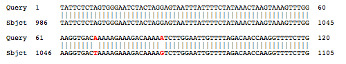
Figure 1. Alignment of a portion of the tomato PSY1 gene between the query sequence for “Red Setter” and the subject sequence for VRT-32-1. The alignment was produced using the NCBI align2seq function in BLAST. Alignment provided by David Francis, The Ohio State University.

Assaying Sequence Variation:

• Conversion to Size Variant (CAP)
• Allele Specific Primer Extension (ASPE)

Additional Resources

For a thorough introduction to molecular markers, see Chapter 3 (p. 45–83), Introduction to Genomics, in:

• Liu, B. H. 1998. Statistical genomics: Linkage, mapping, and QTL analysis. CRC Press, Boca Raton, FL.

For an introduction to molecular markers, linkage mapping, QTL analysis, and marker-assisted selection written for professional plant breeders, see:

• Collard, B.C.Y., M.Z.Z. Jaufer, J. B. Brouwer, and E.C.K. Pang. 2005. An introduction to markers, quantitative trait locus (QTL) mapping and marker-assisted selection for crop improvement: The basic concepts. Euphytica 142: 169–196. (Available online at: http://dx.doi.org/10.1007/s10681-005-1681-5) (verified 29 Dec 2010).

Funding Statement

Development of this page was supported in part by the National Institute of Food and Agriculture (NIFA) Solanaceae Coordinated Agricultural Project, agreement 2009-85606-05673, administered by Michigan State University. Any opinions, findings, conclusions, or recommendations expressed in this publication are those of the author(s) and do not necessarily reflect the view of the United States Department of Agriculture.

PBGworks 879

PBGworks T205,199

PBGworks T203,80

Introduction

Background selection refers to selection applied to regions of the genome that are not known to be associated with desired traits. This type of selection is usually referred to in the context of trait introgression. Trait introgression, the process of integrating a trait from one species into another, is a common strategy used for crop improvement. View an example of introducing bacterial spot resistance to the cultivated tomato.

In the case of tomato, wild species are often used as a source of desirable traits, as there is limited genetic variation within the cultivated tomato. Making crosses (see video below) between cultivated and wild tomato species allows breeders to introduce desirable traits from the wild species. Along with the desired trait from the wild species comes undesired genetic material that the breeder wants to eliminate. This undesired genetic background may, for example, reduce yield or crop quality.

Background Selection Aided by Molecular Markers

Selection against background genomic regions can be greatly facilitated by knowledge of molecular markers. Genotypic data acquired from molecular marker data of mapping populations can be used to create genetic maps so that researchers know the relative distances between molecular markers. Learn more about genetic mapping. If the desired trait has also been mapped, this knowledge can be used to determine which molecular markers located in background regions are linked to the desired traits. This is of particular importance because it can be difficult to remove unwanted linked genetic background. If a genetic map and genotypic data for the population being studied are available, graphical genotypes, can be created. A graphical genotype allows the breeder to visualize the genotype data for each individual. Using graphical genotyping software, breeders can identify individuals with the least unwanted background contribution, as well as individuals with the least linked genetic background. With knowledge of the number of background regions that must be eliminated, breeders can estimate the minimum number of individuals that must be evaluated to obtain at least one individual with fewer (or no) unwanted background regions. Learn more about calculating the minimum number of individuals.

Selecting Against Linked Background

Linked genetic background is generally much more difficult to remove than genetic background on other chromosomes. The probability of removing a portion of linked genetic background depends on the probability of breaking the genetic linkage between the background and desired gene. The probability of breaking the genetic linkage depends on the genetic distance. The greater the genetic distance, the higher the probability that the linkage can be broken. It is therefore important to consider the minimum number of individuals that must be evaluated to help ensure that the linkage will be broken. See a sample calculation of the minimum population size required.

The phenomenon of undesired traits linked to the desired trait being introduced is referred to as linkage drag. Linkage drag has been reported in numerous economically important species, including bean (Miklas, 2007), canola (Cao et al., 2010), potato (Collins et al., 1999), soybean (Warrington et al., 2008), tobacco (Lewis and Rose, 2010), and tomato (Frary et al., 2004). For example, Brouwer et al. (2004) identified QTLs conferring resistance to late blight in tomato. However, they also identified alleles associated with undesirable traits in these regions. To make use of the QTLs conferring late blight resistance, they suggest employing a backcrossing scheme, but without molecular markers tightly linked to late blight resistance and the deleterious alleles, this would be a daunting process. This phenomenon has also been reported in other crop species in the literature. In potato, QTLs conferring late blight resistance have been identified on chromosome V in multiple studies. In all of these studies, the QTL region has also been associated with late maturity and low plant vigor, which are undesirable traits from a breeding perspective (Collins et al., 1999; Oberhagemann et al., 1999; Ewing et al., 2000).

Conclusion

When introgressing desired traits from wild species, background selection must often be applied to help recover the desired background genome. Selection based on molecular marker data and graphical genotypes can be useful to accelerate the background genome recovery process. This is particularly true when desired traits and undesired traits are linked.

References Cited

• Brouwer, D. J., and D. A. St. Clair. 2004. Fine mapping of three quantitative trait loci for late blight resistance in tomato using near isogenic lines (NILs) and sub-NILs. Theoretical and Applied Genetics 108: 628–638 (Available online at: http://dx.doi.org/10.1007/s00122-003-1469-8) (verified 1 June 2012).
• Cao, Z. Y., F. Tian, N. A. Wang, C. C. Jiang, B. Lin, W. Xia, J. Q. Shi, Y. Long, C. Y. Zhang, and J. L. Meng. 2010. Analysis of QTLs for erucic acid and oil content in seeds on A8 chromosome and the linkage drag between the alleles for the two traits in Brassica napus. Journal of Genetics and Genomics 37: 231–240 (Available online at: http://dx.doi.org/10.1016/S1673-8527(09)60041-2) (verified 1 June 2012).
• Collins, A., D. Milbourne, L. Ramsay, R. Meyer, C. Chatot-Balandras, P. Oberhagemann, W. De Jong, C. Gebhardt, E. Bonnel, and R. Waugh. 1999. QTL for field resistance to late blight in potato are strongly correlated with maturity and vigor. Molecular Breeding 5: 387–398. (Availavble online at: http://dx.doi.org/10.1023/A:1009601427062) (verified 1 june 2012).
• Ewing, E. E., I. Simko, C. D. Smart, M. W. Bonierbale, E.S.G. Mizubuti, G. D. May, and W. E. Fry. 2000. Genetic mapping from field tests of qualitative and quantitative resistance to Phytophthora infestans in a population derived from Solanum tuberosum and Solanum berthaultii. Molecular Breeding 6: 25–36. (Availavble online at: http://dx.doi.org/10.1023/A:1009648408198) (verified 1 June 2012).
• Frary, A., T. M. Fulton, D. Zamir, and S. D. Tanksley. 2004. Advanced backcross QTL analysis of a Lycopersicum esculentum x L. pennellii cross and identification of possible orthologs in the Solanaceae. Theoretical and Applied Genetics 108: 485–496 (Available onilne at: http://dx.doi.org/10.1007/s00122-003-1422-x) (verified 1 June 2012).
• Lewis, R. S.,and C. Rose. 2010. Agronomic performance of tobacco mosaic virus-resistant tobacco lines and hybrids possessing the resistance gene N introgressed on different chromosomes. Crop Science 50: 1339–1347 (Available online at: http://dx.doi.org/10.2135/cropsci2009.10.0615) (verified 1 June 2012).
• Miklas, P. N. 2007. Marker-assisted backcrossing QTL for partial resistance to sclerotinia white mold in dry bean. Crop Science 47: 935–942 (Available online at: http://dx.doi.org/10.2135/cropsci2006.08.0525) (verified 1 June 2012).
• Oberhagemann, P., C. Chatot-Balandras, R. Schafer-Pregl, D. Wegener, C. Palomino, F. Salamini, E. Bonnel, and C. Gebhardt. 1999. A genetic analysis of quantitative resistance to late blight in potato: Towards marker-assisted selection. Molecular Breeding 5: 399–415. (Availavble online at: http://dx.doi.org/10.1023/A:1009623212180) (verified 4 June 2012).
• Warrington, C. V., S. Zhu, W. A. Parrott, J. N. All, and H. R. Boerma. 2008. Seed yield of near-isogenic soybean lines with introgressed quantitative trait loci conditioning resistance to corn earworm (Lepidoptera: Noctuidae) and soybean looper (Lepidoptera: Noctuidae) from PI 229358. Journal of Economic Entomology 101: 1471–1477. (Availavble online at: http://dx.doi.org/10.1603/0022-0493(2008)101[1471:SYONSL]2.0.CO;2) (verified 1 June 2012).

External Links

• Shermin, J.,and D. Quinn. Genetic mapping [Online lesson]. Wheat CAP: Wheat Coordinated Agricultural Project. Available at: http://maswheat.ucdavis.edu/Education/animations/anim_mapping.htm (verified 1 June 2012).

Funding Statement

Development of this page was supported in part by the National Institute of Food and Agriculture (NIFA) Solanaceae Coordinated Agricultural Project, agreement 2009-85606-05673, administered by Michigan State University. Any opinions, findings, conclusions, or recommendations expressed in this publication are those of the author(s) and do not necessarily reflect the view of the United States Department of Agriculture.

PBGworks 772

Presenter: Christine Hackett, Biomathematics and Statistics Scotland, Dundee, UK.

This workshop is in two parts: linkage analysis, and QTL mapping. The first part is an overview of the theory of segregation analysis and linkage analysis in an autotetraploid species, such as potato, followed by a demonstration of the software program TetraploidMap for Windows on some potato marker data from the cross Stirling x 12601ab1. The second part is an overview of QTL mapping in an autotetraploid species, followed by a demonstration of how to perform QTL mapping using TetraploidMap for Windows and how to compare different QTL models.

You can view the webinar below or at the SolCAP website.

If you experience problems viewing this video connect to our YouTube channel or see the YouTube troubleshooting guide.

View other SolCAP webinars

External Links

• Hackett, C. 2010. Linkage analysis and QTL mapping in tetraploids [Online seminar]. Solanaceae Coordinated Agricultural Project. Available at: http://solcap.msu.edu/linkage_analysis_webinar.shtml (verified: 11 May 2012).

Funding Statement

Development of this page was supported in part by the National Institute of Food and Agriculture (NIFA) Solanaceae Coordinated Agricultural Project, agreement 2009-85606-05673, administered by Michigan State University. Any opinions, findings, conclusions, or recommendations expressed in this publication are those of the author(s) and do not necessarily reflect the view of the United States Department of Agriculture.

PBGworks 878

This module provides an example of using analysis of variance (ANOVA) to assess differences in tomato bacterial spot resistance due to molecular marker genotype (treatment effect) to determine whether genotype of each molecular marker results in differences in disease severity in a BC₁ population.

The following links provide:

• The example
• The dataset
• The SAS output

SAS Code

The SAS code is presented in two ways:

• As a screenshot taken from SAS after the code has been entered (Fig.1)
• As plain text

Figure 1. SAS Screenshot taken after SAS code for analysis of variance in a balanced population was entered. Screenshot credit: David Francis, The Ohio State University.

Plain Text SAS Code

data map;
     infile ‘a:\lnkspt.csv’; delimiter = “,” firstobs = 4;
     input gen vsc pop tg23 pto;
proc sort;
     by tg23;
proc glm;
     class tg23;
     model pop = tg23;
     means tg23 / lsd lines;
proc sort;
     by pto;
proc glm;
     class pto;
     model pop = pto;
     means pto / lsd lines;
run;

Funding Statement

Development of this page was supported in part by the National Institute of Food and Agriculture (NIFA) Solanaceae Coordinated Agricultural Project, agreement 2009-85606-05673, administered by Michigan State University. Any opinions, findings, conclusions, or recommendations expressed in this publication are those of the author(s) and do not necessarily reflect the view of the United States Department of Agriculture.

PBGworks 906

Introduction

Population size, structure, and the number of molecular markers genotyped can have significant impacts on quantitative trait locus (QTL) detection. This page focuses on the effect population size can have on QTL detection. Prior knowledge of theories regarding the genetics controlling the trait can help guide breeders as to the number of plants required to detect QTLs of various sizes using the following equation. Solving the equation below can help breeders optimize resources while still gaining the desired outcome.

Equation to Calculate Minimum Sample Size

Using units of phenotypic standard deviations, sample sizes can be estimated using the following equations:

For an F₂ population,

N_F2 = [1 – r²_F2 / r²_F2] x {[z_{(1 – (α / 2))} / (1 – r²_F2)^1/2] + z_{(1 – β)}}² x [1 + (k² / 2)]

For a BC₁ population,

N_BC1 = [1- r²_BC1 / r²_BC1 ] x {[z _{(1 – (α / 2))} /(1 – r²_BC1)^1/2 ] + z_{(1 – β)}}² x [1 + (k² / 2)]

In these equations,

• r² is the fraction of phenotypic variance explained by the QTL. Note that r² is valid only for simple models. Mean Squares provide an alternative method to estimate fraction of phenotypic variation when models have replication and location.
• k is the dominance coefficient (k = 0 for completely additive trait, k = 1 for completely dominant trait and k = -1 for completely recessive trait). This equation assumes that the marker and QTL are coincidental.
• α is the type I error (the probability of incorrectly identifying an association that does not, in fact, exist)
• β is the type II error (the probability of failing to identify a true association)
• From normal distribution tables:
  • z_(1-(α/2)) = 1.96 at α = 0.05
  • z_(1–β) = 1.28 at ß = 0.10

For example, in an F₂ population, the estimated sample size required to detect a dominant QTL that is responsible for 30% of the phenotypic variation is 46.

N_F2 = [(1 – 0.30) / 0.30] x {[1.96 / (1 – 0.30)^1/2] + 1.28}² x [1 + (1² / 2)] = 46

Funding Statement

Development of this lesson was supported in part by the National Institute of Food and Agriculture (NIFA) Solanaceae Coordinated Agricultural Project, agreement 2009-85606-05673, administered by Michigan State University. Any opinions, findings, conclusions, or recommendations expressed in this publication are those of the author(s) and do not necessarily reflect the view of the United States Department of Agriculture.

PBGworks 862

This module provides an example of using analysis of variance (ANOVA) to assess differences in tomato bacterial spot resistance due to molecular marker genotype (treatment effect) in a BC₁ population.

The following links provide:

• The example
• The dataset
• The SAS program

Funding Statement

Development of this page was supported in part by the National Institute of Food and Agriculture (NIFA) Solanaceae Coordinated Agricultural Project, agreement 2009-85606-05673, administered by Michigan State University. Any opinions, findings, conclusions, or recommendations expressed in this publication are those of the author(s) and do not necessarily reflect the view of the United States Department of Agriculture.

PBGworks 907

Introduction

Molecular markers have great potential to assist breeders in developing improved varieties by complementing phenotypic selection. They work by either measuring directly or indirectly a specific DNA sequence difference between various genotypes. When these markers are found to be linked to a trait of interest, it can aid the breeder in more efficiently selecting the plants or lines to move forward in the program (forward selection). Markers can also be used to improve all other trait combinations in the germplasm, either by crossing out unwanted alleles or maintaining those of value (background selection). This module is structured to give an overview of the traditional view of molecular markers; as bands on a gel. Therefore, traditional markers indirectly measure DNA differences. With advances in DNA sequencing techniques, the cost of directly determining the sequence of a DNA fragment has dropped considerably. As a result, newer molecular marker tools are quickly becoming more common and are more effective in meeting plant breeding needs on a large scale. However, not all laboratories can currently afford to invest in the equipment required to take advantage of newer technologies and the newer technologies may not be more efficient on a small scale. You can also learn about this alternative view of molecular markers, where marker data is typically presented to breeders as fluorescence intensity values. This alternative view includes information about single nucleotide polymorphism (SNP) markers.

To understand the concepts behind any molecular marker system first requires an understanding of DNA and its structure, including the nucleotides and DNA base pairing.

• See an example of molecular markers being used to breed for tomatoes with improved resistance to bacterial spot.

Traditional View of Molecular Markers

This list of traditional molecular markers including their acronyms can give us some idea of the basis of the molecular marker. It also describes the differences (polymorphisms) in DNA sequences they target.

Isozyme: By measuring variations in enzymes, isozyme analysis exploits differences in the genes that code for or regulate enzyme synthesis or activity.

RFLP (Restriction Fragment Length Polymorphism): Indirectly measure DNA sequence differences based upon the varying lengths of DNA fragments resulting from cutting it with restriction enzymes. These “fragment length polymorphisms” are visualized by hybridizing the cut DNA with labeled probes from DNA libraries.

RAPD (Random Amplified Polymorphic DNA): Utilizing a large number of short DNA primers with varying sequences, this technique exploits differences in the primer binding sites as different DNA will be amplified by the polymerase chain reaction (PCR).

AFLP (Amplified Fragment Length Polymorphism): Utilizing restriction enzymes and a large number of short DNA primers with varying sequences, this technique exploits differences in the primer binding sites as different DNA will be amplified using PCR.

SSR (Simple Sequence Repeat) or microsatellite: Using PCR, this technique exploits differences in short repetitive sequences (e.g., CAA vs. CAACAACAA) by using specifically designed DNA primers that bind on each side of repetitive DNA sequences.

SCAR (Sequence Characterized Amplified Region): Exploit length differences between two PCR products (not necessarily repeats) by using specifically designed DNA primers that bind on each side of a difference in DNA sequence. These are often created by sequencing RAPD marker PCR products and then designing more specific DNA primers than are used for the original RAPD markers.

CAP (Cut/Cleaved Amplified Polymorphism): Exploit differences in DNA sequences between two PCR products based on the presence or absence of restriction enzyme cutting sites. These markers are often designed from RFLP markers.

Steps to Marker Detection

Each marker is detected differently, which allows us to look at the different types of variation listed above.

Isozyme: separate by starch gel and stain

RFLP: digest with restriction enzyme (RE), separate by agarose gel electrophoresis, transfer DNA to membrane, hybridize with labeled probe, visualize by autoradiography

RAPD: amplify by PCR, separate by agarose gel electrophoresis, visualize with Ethidium Bromide (EtBr) stain

AFLP: digest with RE, ligate to linker, amplify by PCR with labeled primer, separate by polyacrylamide gel electrophoresis, visualize by autoradiography

SSR: amplify by PCR, separate by agarose gel electrophoresis, visualize with EtBr stain

SCAR: amplify by PCR, separate by agarose gel electrophoresis, visualize with EtBr stain

CAP: amplify by PCR, digest with RE, separate by agarose gel electrophoresis, visualize with EtBr stain

Looking at the steps to marker detection can help us figure out how easy or difficult it may be to genotype using a particular molecular marker. For example, RFLP markers require a lot of steps and they also require steps that none of the other markers do, in particular creating a library of DNA or cDNA probes. This suggests that RFLPs take very specialized knowledge and laboratory skills to perform. People who have worked with RFLPs can tell you this is true! They likely prefer to work with markers that are PCR-based because once you have learned the PCR technique, you can work with many different types of molecular markers and PCR does not take long. Table 1 provides us with some more information to help us compare the different molecular markers. We know that PCR-based markers are advantageous, but the table provides us with some information we wouldn’t necessarily know based on the marker names or the detection steps alone. The additional resources listed at the end of this page can provide you with more in-depth information about these molecular markers.

Additional Resources

For a further introduction to molecular markers, see Chapter 3 (p. 45–83), Introduction to Genomics, in:

• Liu, B. H. 1998. Statistical genomics: Linkage, mapping, and QTL analysis. CRC Press, Boca Raton, FL.

For an introduction to molecular markers, linkage mapping, QTL analysis, and marker-assisted selection written for professional plant breeders, see:

• Collard, B.C.Y., M.Z.Z. Jaufer, J. B. Brouwer, and E.C.K. Pang. 2005. An introduction to markers, quantitative trait locus (QTL) mapping and marker-assisted selection for crop improvement: The basic concepts. Euphytica 142: 169–196. (Available online at: http://dx.doi.org/10.1007/s10681-005-1681-5) (verified 24 Mar 2012).

Funding Statement

Development of this page was supported in part by the National Institute of Food and Agriculture (NIFA) Solanaceae Coordinated Agricultural Project, agreement 2009-85606-05673, administered by Michigan State University. Any opinions, findings, conclusions, or recommendations expressed in this publication are those of the author(s) and do not necessarily reflect the view of the United States Department of Agriculture.

PBGworks 856

Introduction

Pyramiding genes on the same chromosome is a special case of gene pyramiding. This case study describes the use of molecular markers to pyramid two disease resistance genes on tomato chromosome 5: Rx-3 (resistance to tomato bacterial spot) and Pto (resistance to bacterial speck).

Bacterial spot and bacterial speck, two diseases with worldwide economic importance, can impact tomato crops simultaneously. Figure 1 shows a field affected by bacterial spot. Yang and Francis (2005) sought to combine resistance genes for both diseases. Although Yang and Francis (2005) knew from previous studies (Yang et al., 2005; Martin et al., 1993) that both resistance genes were on chromosome 5, they didn’t know the genetic distance between the two genes.

To combine Rx-3 and Pto, Yang and Francis (2005) crossed two inbred parents (see video): one homozygous for Rx-3 but susceptible to bacterial speck and the other homozygous for Pto but susceptible to bacterial spot. The video below outlines the general procedure for making crosses. The F₁ progeny were self-pollinated to obtain F₂ seed.

Figure 1. Tomato plot that includes tomato plants that are resistant (left) and susceptible (mid-right) to bacterial spot. Photo courtesy of David Francis, The Ohio State University.

In the F₂ generation, Yang and Francis (2005) wanted to identify individuals resistant to bacterial spot and bacterial speck, and to calculate the genetic distance between Rx-3 and Pto. To achieve these objectives, Yang and Francis (2005) genotyped a population of 419 individuals with two molecular markers (one associated with Pto and one associated with Rx-3) to identify individuals with alleles that confer resistance to both diseases. In the case of Pto, the molecular marker was within the Pto gene, so Francis and Yang did not have to worry about recombination between the marker and gene. However, in the case of Rx-3, the molecular marker used to select for bacterial spot resistance was not within Rx-3, so recombination between the marker and Rx-3 was possible. This meant that selection based on the marker alone wouldn’t be perfect. In some cases, individuals with the resistant allele would be susceptible. Yang and Francis conducted phenotypic screenings to confirm that individuals expected to be resistant based on their genotype were, in fact, resistant.

Individuals with resistance to both bacterial spot and bacterial speck could only be obtained if a recombination event occurred between Pto and Rx-3, because each parent carried only one of the resistance genes. The chance of a recombination event depends on the genetic distance between Pto and Rx-3. Of the 419 F₂ individuals genotyped, Yang and Francis identified 13 plants that were homozygous for bacterial spot and bacterial speck resistance alleles and 94 individuals that were heterozygous.

Yang and Francis estimated that Pto and the Rx-3 marker were 36.8 ± 2.2 cM apart. See the animation about genetic mapping to learn more about the principles of genetic mapping. The loose linkage between Pto and the Rx-3 marker means that breeders must take care to ensure that they maintain resistance conferred by Pto and Rx-3 when making crosses with individuals that have both these resistance genes.

References Cited

• Martin, G. B., M. C. de Vicente, and S. D. Tanksley. 1993. High-resolution linkage analysis and physical characterization of the PTO bacterial-resistance locus in tomato. Molecular Plant-Microbe Interactions 6: 26–34. (Available online at: http://www.apsnet.org/publications/mpmi/BackIssues/Documents/1993Abstracts/Microbe06-026.htm) (verified 30 Aug 2012).
• Yang, W., and D. M. Francis. 2005. Marker-assisted selection for combining resistance to bacterial spot and bacterial speck in tomato. Journal of the American Society for Horticultural Science 130: 716–721. (Available online at: http://journal.ashspublications.org/cgi/content/abstract/130/5/716) (verified 30 Aug 2012).
• Yang, W. C., E. J. Sacks, M.L.L. Ivey, S. A. Miller, and D. M. Francis. 2005. Resistance in Lycopersicum esculentum intraspecific crosses to race T1 strains of Xanthomonas campestris pv. vesicatoria causing bacterial spot of tomato. Phytopathology 95: 519–527. (Available online at: dx.doi.org/10.1094/PHYTO-95-0519) (verified 30 Aug 2012).

External Links

• Shermin, J., and D. Quinn. Genetic mapping [online lesson] Wheat CAP: Wheat Coordinated Agricultural Project. Available at: http://maswheat.ucdavis.edu/Education/animations/anim_mapping.htm (verified 30 Aug 2012).

Funding Statement

Development of this page was supported in part by the National Institute of Food and Agriculture (NIFA) Solanaceae Coordinated Agricultural Project, agreement 2009-85606-05673, administered by Michigan State University. Any opinions, findings, conclusions, or recommendations expressed in this publication are those of the author(s) and do not necessarily reflect the view of the United States Department of Agriculture.

PBGworks 903